Bayes for Beginners 2: The Prior

In his inaugural Presidential Column, APS President C. Randy Gallistel introduced beginners to Bayesian statistical analysis. This month, he continues the introduction to Bayes with a lesson on using prior distributions to improve parameter estimates.

In last month’s column, I focused on the distinction between likelihood and probability.

To review, probability attaches to the possible outcomes from a random process like coin flipping (known technically as a Bernoulli process). A probability distribution gives the probabilities for the different possible results given the parameters of the process. Suppose we are given a 50% chance of success (i.e., of flipping a head; p = .5) and told that there were 10 flips. Given these parameters, the probability of getting exactly 5 heads when flipping a coin 10 times is roughly .25.

Likelihood, by contrast, attaches to our parameter estimates and to our hypotheses. For example, given that we have observed 9 heads in 10 flips of a coin, the likelihood that the probability of flipping a head is 50% (i.e., that p = .5) is very low. The likelihood that p = .9 is greater by a factor of almost 40. The likelihood function tells us the relative likelihoods of the different possible values for p.

The likelihood function is only one of two components of a Bayesian calculation, however. The other is the prior, which is necessary for estimating parameters and for drawing statistical conclusions. Using prior distributions improves one’s parameter estimates and quantifies one’s hypotheses.

A prior distribution can and should take account of what one already knows. However, when one knows very little, one can use the Jeffreys priors, named after English mathematician Sir Harold Jeffreys, who helped revive the Bayesian view of probability. Jeffreys priors are some of the most interesting and useful prior distributions, and they derive from the mathematical implications of knowing absolutely nothing about the parameters one wants to estimate other than their possible ranges.

Improving Parameter Estimates With a Prior

A prior distribution assigns a probability to every possible value of each parameter to be estimated. Thus, when estimating the parameter of a Bernoulli process p, the prior is a distribution on the possible values of p. Suppose p is the probability that a subject has done X. Assume we initially have no idea how widespread this practice is. We ask the first three subjects whether they have done it. They all say, “No.” At this early stage, what proportion of the population should we estimate has done X? And how certain should we be about our estimate?

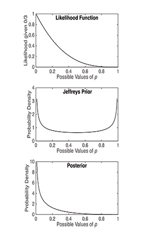
The data by themselves give p(X) = 0. That value specifies a distribution with no variance; it predicts that every subsequent subject also will not have done X. Our intuition suggests that it is unwise to take three people’s experiences as representative of all people’s experiences. The data at hand, however, do give us some information: We already know that p(X) ≠ 1 (because at least one subject has not done X), and it seems unlikely that p(X) > .9 (because none of our three subjects have done X).

Bayesian parameter estimation rationalizes and quantifies these intuitions by bringing a prior distribution into the calculation. The prior distribution represents uncertainty about the value of the parameters before we see data. Jeffreys realized that knowing nothing about a parameter other than its possible range (in this case, 0–1) often uniquely specifies a prior distribution for the estimation of that parameter.

The Jeffreys prior for the p parameter of a Bernoulli process is in the form called the beta distribution. The beta distribution itself has two parameters, denoted a and b. For the Jeffreys prior, these take the values a = b = .5. Following the common practice, I call these parameters hyperparameters to distinguish them from the parameter of the distribution that we are trying to estimate.

By adopting a Jeffreys prior, we can calculate a best estimate for p and quantify our current uncertainty about p at every stage of data gathering, from the stage where we have no data to the stage where we have an n in the millions. The Bayesian calculation requires multiplying the likelihood function by the prior distribution and normalizing the result in order to obtain the posterior distribution (i.e., a new distribution of probabilities for the different values of p, taking into account the data and the prior). This process sounds pretty intimidating.

When we use the Jeffreys prior, however, the posterior distribution takes the same form as the prior distribution; a beta distribution goes in as the prior and a beta distribution emerges as the posterior. (A prior distribution with this wonderful property is called a conjugate prior.) Thus, the only thing that the computation does is change the values of the parameters of a beta distribution. Moreover, the computation of the new values for these parameters is very simple: a_post = a_prior + n_s and b_post = b_prior + n_f , where n_s denotes the number of successes (in this case, subjects who have done X) and n_f the number of failures (subjects who haven’t). The best estimate of p — the mean of the posterior distribution — is a_post / (a_post +  b_post). Statistical calculations never get easier than that.

Best of all, the resulting posterior distribution tells us how uncertain we should be about the true value of p. In traditional statistics, this is what the confidence interval is supposed to do. (It does it badly, but that’s another story.) Estimating a confidence interval for estimates of p when the sample is low is not straightforward, whereas the calculation of the posterior distribution using a conjugate prior is, as already explained, simplicity itself.

Figure 1 plots the likelihood function, the Jeffreys prior, and the posterior distribution for the case where we have three negatives and no positives. Notice how well Bayesian statistics can capture what our intuition tells us we can learn from this small sample.